Tutorial: Visualizing genomic tracks with Gviz
Published:
This tutorial covers plotting of track files such as bigWig files for better visualization. It was originally written in December 2019 for the Laboratory of Cell Systems, Institute for Protein Research, Suita, Osaka, Japan.
The data used here are ChIP-seq bigWig files (Med1 and H3K27Ac respectively) obtained from the following papers:
- Kagey MH et al., Mediator and cohesin connect gene expression and chromatin architecture. Nature 467, 430–435 (2010).
- Creyghton et al., Histone H3K27ac separates active from poised enhancers and predicts developmental state. PNAS 107, 21931–21936 (2010).
Setting up
Load the libraries.
library(tidyverse)
library(Gviz)
library(rtracklayer)
library(GenomicFeatures)
Then we have to make a TxDb object from the GTF annotation.
GTF_dir <- "D:/Rmd_compilations/20191226_gviz/Mus_musculus.GRCm38.98.chr.gtf"

# mm10_txdb <- makeTxDbFromGFF(GTF_dir,
#                              format    = "gtf",
#                              organism  = "Mus musculus",
#                              dbxrefTag = "gene_name")
#
# saveDb(mm10_txdb, "mm10.txdb")

mm10_txdb <- loadDb("D:/Rmd_compilations/20191226_gviz/mm10.txdb")
Plotting the gene region
Because we are using an Ensembl GTF file, turn off the UCSC chromosome name check.
options(ucscChromosomeNames = FALSE)
Then we read the genome axis track and the track for the region of interest.
# read the genome axis, there is no need to pass any argument
gtrack <- GenomeAxisTrack()

# specify the start and end of the region
# (this has to be decided after looking at IGV)
chr_no    <- "12"      # chromosome number
chr_start <- 86330000  # start of region
chr_end   <- 86583978  # end of region

gtTrack <- GeneRegionTrack(
  mm10_txdb,
  chromosome            = chr_no,
  start                 = chr_start,
  end                   = chr_end,
  transcriptAnnotation  = "gene_id",  # "symbol" gives the gene symbol
  fontsize.group        = 20          # free to adjust font size
)
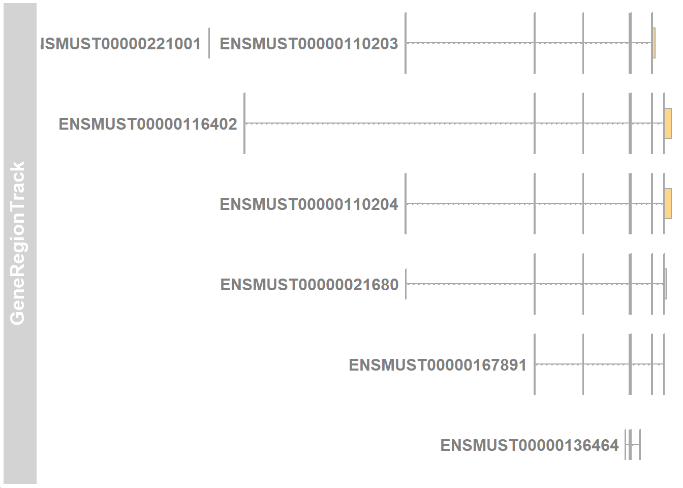
Try plotting the track.
plotTracks(gtTrack)
Plotting the ideogram track
The ideogram track shows the position of the region within the chromosome. This function automatically downloads annotation from a database, so we need to give the chromosome name in UCSC naming (with the chr prefix). After retrieving the information, we convert it back to the naming without the prefix.
itrack <- IdeogramTrack(
  genome     = "mm10",
  chromosome = paste0("chr", chr_no),  # specify chromosome in UCSC naming
  from       = chr_start,
  to         = chr_end
)

itrack@chromosome <- chr_no

# remove "chr" from the chromosome naming
levels(itrack@bandTable$chrom) <- sub(
  "^chr", "", levels(itrack@bandTable$chrom), ignore.case = TRUE
)
Importing and plotting the bigWig files
Now we import the bigWig files for the data we want.
For Ensembl annotation the chromosome is named 1 instead of chr1, so the chr string has to be removed. The important thing is to have a consistent chromosome naming scheme (with or without chr) across all annotation. In this tutorial I remove all the chr strings.
bw_med1 <- import.bw("D:/Rmd_compilations/20191226_gviz/Med1.bigwig", as = "GRanges")
bw_h3k  <- import.bw("D:/Rmd_compilations/20191226_gviz/H3K27Ac.bigwig", as = "GRanges")

# change chromosome names to drop "chr" (this depends on the data)
bw_med1@seqnames@values <- str_replace_all(bw_med1@seqnames@values, "chr", "") %>% as.factor()
bw_h3k@seqnames@values  <- str_replace_all(bw_h3k@seqnames@values, "chr", "") %>% as.factor()

bw_med1@seqinfo@seqnames <- str_replace_all(bw_med1@seqinfo@seqnames, "chr", "")
bw_h3k@seqinfo@seqnames  <- str_replace_all(bw_h3k@seqinfo@seqnames, "chr", "")
Then we specify which part of the data we want to show.
# track 1: Med1
med1_track <- DataTrack(
  range          = bw_med1,
  chromosome     = chr_no,
  from           = chr_start,
  to             = chr_end,
  ylim           = c(0, 290),
  col.histogram  = c("#FDE725FF")
)

# track 2: H3K27Ac
h3k_track <- DataTrack(
  range          = bw_h3k,
  chromosome     = chr_no,
  from           = chr_start,
  to             = chr_end,
  ylim           = c(0, 240),
  col.histogram  = c("#440154FF")
)
Before plotting the tracks, we convert the gene IDs to gene symbols.
convertensembl <- function(x = gtTrack) {
  require(biomaRt)
  require(org.Mm.eg.db)

  mouse <- useMart("ensembl", dataset = "mmusculus_gene_ensembl")

  convertedgene <- getBM(
    attributes = c("ensembl_gene_id", "external_gene_name"),
    filters    = "ensembl_gene_id",
    values     = x@range@elementMetadata@listData$gene,
    mart       = mouse
  )

  for (i in 1:nrow(convertedgene)) {
    x@range@elementMetadata@listData$gene <- x@range@elementMetadata@listData$gene %>%
      str_replace_all(convertedgene[i, 1], convertedgene[i, 2])
  }
  return(x)
}

# convert Ensembl IDs to gene names
gtTrack <- convertensembl(gtTrack)
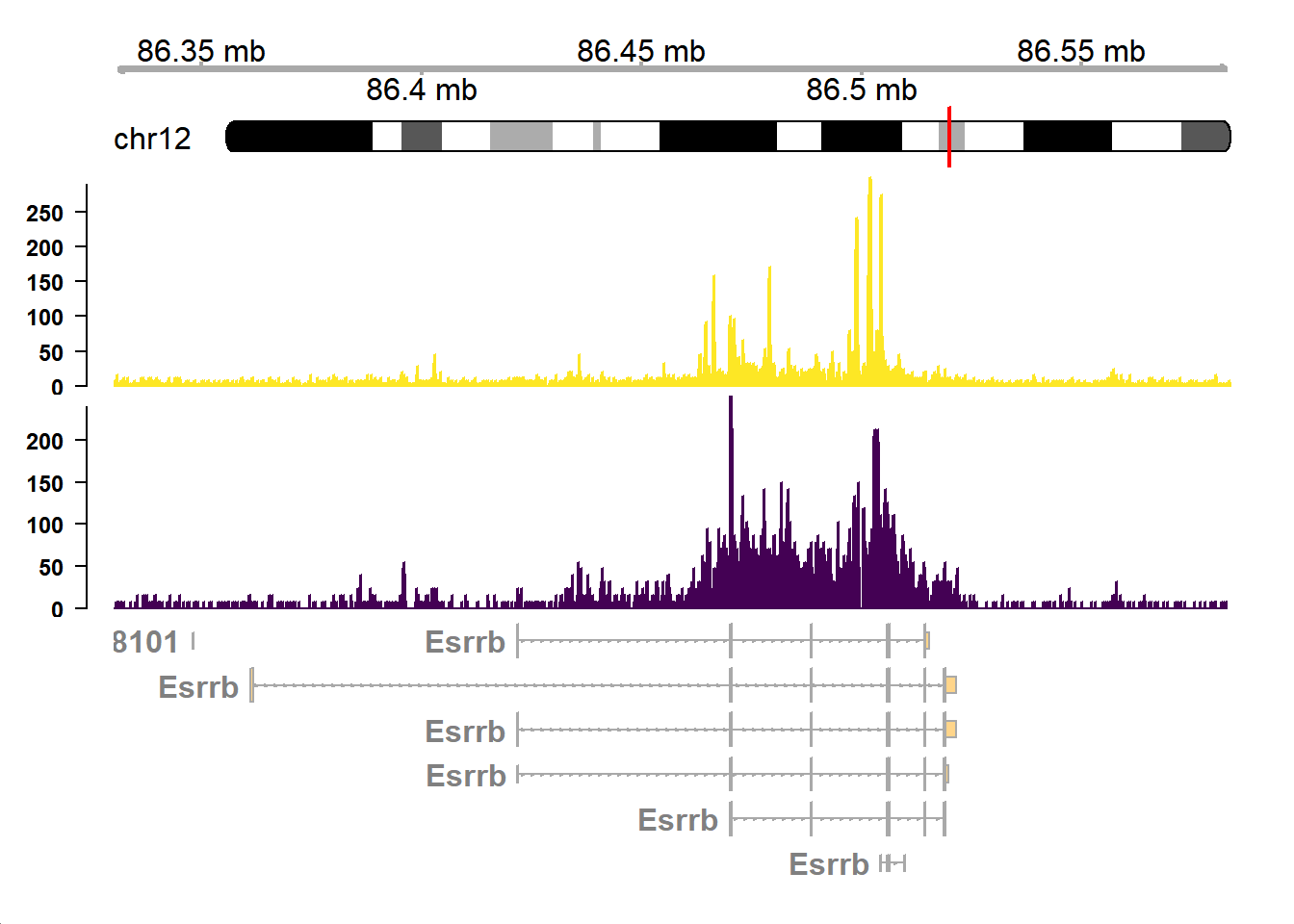
Plotting all tracks together
Finally, combine the tracks.
combinetracks <- plotTracks(
  c(gtrack, itrack, med1_track, h3k_track, gtTrack),
  transcriptAnnotation = "gene",
  type                 = "hist",
  from                 = chr_start,
  to                   = chr_end,
  background.title     = "white",
  fontcolor            = "black",
  col.axis             = "black",
  fontsize             = 15,
  showTitle            = FALSE,
  margin               = 40,
  innerMargin          = 10
)